The Scientist and Engineer's Guide to
Digital Signal Processing
By Steven W. Smith, Ph.D.
Book Search

Table of contents
- 1: The Breadth and Depth of DSP
- 2: Statistics, Probability and Noise
- 3: ADC and DAC
- 4: DSP Software
- 5: Linear Systems
- 6: Convolution
- 7: Properties of Convolution
- 8: The Discrete Fourier Transform
- 9: Applications of the DFT
- 10: Fourier Transform Properties
- 11: Fourier Transform Pairs
- 12: The Fast Fourier Transform
- 13: Continuous Signal Processing
- 14: Introduction to Digital Filters
- 15: Moving Average Filters
- 16: Windowed-Sinc Filters
- 17: Custom Filters
- 18: FFT Convolution
- 19: Recursive Filters
- 20: Chebyshev Filters
- 21: Filter Comparison
- 22: Audio Processing
- 23: Image Formation & Display
- 24: Linear Image Processing
- 25: Special Imaging Techniques
- 26: Neural Networks (and more!)
- 27: Data Compression
- 28: Digital Signal Processors
- 29: Getting Started with DSPs
- 30: Complex Numbers
- 31: The Complex Fourier Transform
- 32: The Laplace Transform
- 33: The z-Transform
- 34: Explaining Benford's Law
How to order your own hardcover copy
Wouldn't you rather have a bound book instead of 640 loose pages?Your laser printer will thank you!
Order from Amazon.com.
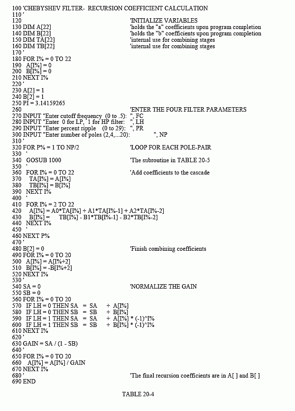
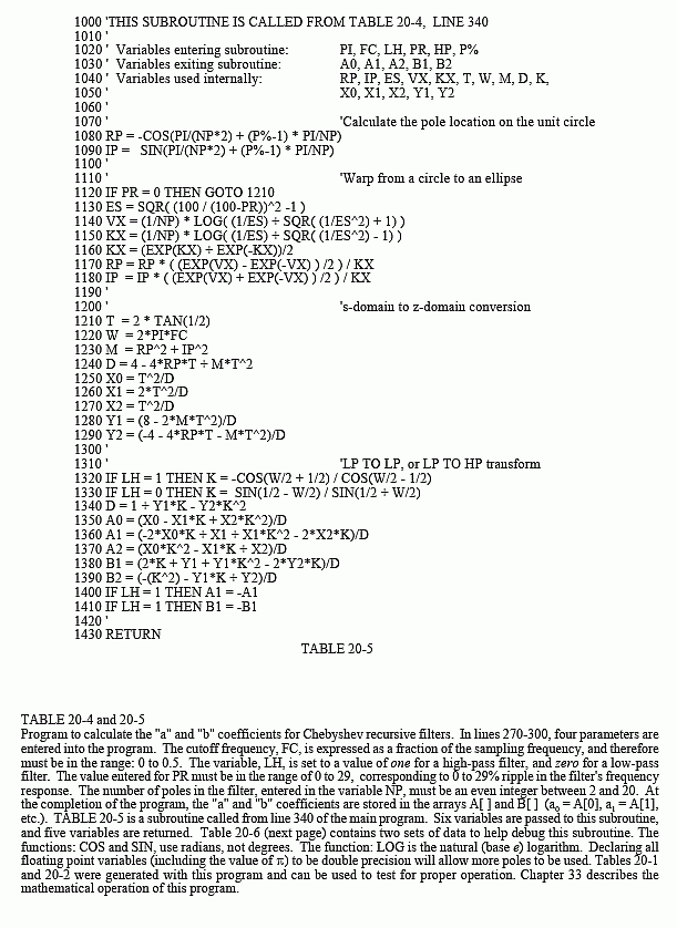
Chapter 20: Chebyshev Filters
The main limitation of digital filters carried out by convolution is execution time. It is possible to achieve nearly any filter response, provided you are willing to wait for the result. Recursive filters are just the opposite. They run like lightning; however, they are limited in performance. For example, consider a 6 pole, 0.5% ripple, low-pass filter with a 0.01 cutoff frequency. The recursion coefficients for this filter can be obtained from Table 20-1:
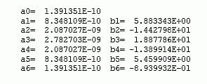
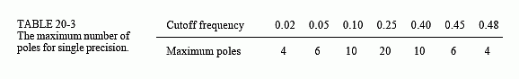
Look carefully at these coefficients. The "b" coefficients have an absolute value of about ten. Using single precision, the round-off noise on each of these numbers is about one ten-millionth of the value, i.e., 10-6. Now look at the "a" coefficients, with a value of about 10-9. Something is obviously wrong here. The contribution from the input signal (via the "a" coefficients) will be 1000 times smaller than the noise from the previously calculated output signal (via the "b" coefficients). This filter won't work! In short, round-off noise limits the number of poles that can be used in a filter. The actual number will depend slightly on the ripple and if it is a high or low-pass filter. The approximate numbers for single precision are:
The filter's performance will start to degrade as this limit is approached; the step response will show more overshoot, the stopband attenuation will be poor, and the frequency response will have excessive ripple. If the filter is pushed too far, or there is an error in the coefficients, the output will probably oscillate until an overflow occurs.
There are two ways of extending the maximum number of poles that can be used. First, use double precision. This requires using double precision in the coefficient calculation as well (including the value for pi ).
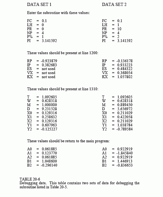
The second method is to implement the filter in stages. For example, a six pole filter starts out as a cascade of three stages of two poles each. The program in Table 20-4 combines these three stages into a single set of recursion coefficients for easier programming. However, the filter is more stable if carried out as the original three separate stages. This requires knowing the "a" and "b" coefficients for each of the stages. These can be obtained from the program in Table 20-4. The subroutine in Table 20-5 is called once for each stage in the cascade. For example, it is called three times for a six pole filter. At the completion of the subroutine, five variables are return to the main program: A0, A1, A2, B1, & B2. These are the recursion coefficients for the two pole stage being worked on, and can be used to implement the filter in stages.